By Wolf-D. Ihlenfeldt, Xemistry GmbH
In February 2013, a question was posted on the Blue Obelisk forum:
I want the adjacency matrix representation of a molecule. Given an MDL Molfile or SDF file, I would like to obtain a adjacency matrix for each molecule as below. All atom are considered vertices, all bonds as edges. If two vertices i and j are connected by single, double or triple bond then the A_ij entry of the adjacency matrix should be 1, 2, and 3 respectively.
Are there any open source program that facilitate this and further analysis on the matrix like calculating the distance distribution, distance matrix, matrix based topological descriptors etc ? I would prefer Python or Java based program.
Well, we cannot give you Python or Java solutions, but the problem is trivial to address with the Cactvs toolkit.
The standard form of the adjacency matrix stores bond orders in the i/j elements, a zero value if the two atoms are not directly connected by a bond, and the VB free electron count in the diagonal. This was a popular structure representation in the early days of chemical computing, especially in languages such as Fortran77 which do not support pointers, lists, and other modern programming language elements. Space-wise, this is of course not a good solution, because the required memory increases with the square number of atoms in the structure.
Computing the matrix is straightforward. Since this is a rather basic item, and may be useful in later projects, it is a good idea to encapsulate its computation as a property definition. This is done by firing up the toolkit property editor (it is an integral part of the factory program, or use its stand-alone variant), name it (we use E_ADJACENCY_MATRIX, with an E prefix since this is a property of an ensemble object), define its datatype (integer matrix), and add a simple Tcl-script computation function. This is the encapsulated property definition file. The embedded computation function is this:
proc CSgetE_ADJACENCY_MATRIX {eh} {
    set m {}
    foreach a1 [ens atoms $eh anormal] {
        set row {}
        foreach a2 [ens atoms $eh anormal] {
            if {$a1==$a2} {
                lappend row [atom get $eh $a1 A_FREE_ELECTRONS]
            } else {
                set b [bond bond $eh [list $a1 $a2]]
                if {$b=="" || [bond get $eh $b B_TYPE]!="normal"} {
                    lappend row 0
                } else {
                    lappend row [bond get $eh $b B_ORDER]
                }
            }
        }
        lappend m $row
    }
    ens set $eh E_ADJACENCY_MATRIX $m
}
It is simply a pair of nested loops over all atoms. For maximum flexibility, atoms which are not simple elements are filtered out by the anormal filter. Bonds which are not simple VB bonds are also ignored by checking the value of the B_TYPE property. The matrix is set up as a nested row-oriented list - this is what the parser for inputting the matrix from a Tcl representation expects. When the ens set command is executed, the Tcl form the function set up is decoded, and the property attached in its internal binary representation to the ensemble object.
The bond bond command may appear cryptic, but it is actually a completely logical form of the general minor object label retrieval machinery of the toolkit. Minor object label retrieval commands return the labels of found objects, or an empty result if nothing is t found. Minor objects which should be located can be specified in multiple fashions. For bonds, a popular form is a combination of the ensemble handle and a list of the labels of all the atoms participating in it. We already have two atoms from the atom list iterators - we use these, in arbitrary order, to obtain the bond label if a bond between the atoms exists, or an empty string if no such bond is found. There are many other ways to identify a specific bond - directly by its label in combination with the ensemble handle, as in the other bond commands of this function, by bond list indices counted from the beginning or end of the bond list, by reference to backup bond labels which were automatically saved prior to an operation which changed the bond labels, by equality comparison with arbitrary bond properties, or by a few magic identifiers such as first, last, or random. Using bond bond with a bond label instead of an atom label pair or another more complex identification is absolutely possible, but of course pointless, since the same label is always returned.
Here is an interactive session showing the straightforward use of the new property with a sample molecule (ethanol, with all hydrogens):
cactvs>molfile read ethanol.mol
ens0
cactvs>ens get ens0 E_ADJACENCY_MATRIX
{0 1 0 1 1 1 0 0 0} {1 0 1 0 0 0 1 1 0} {0 1 4 0 0 0 0 0 1} {1 0 0 0 0 0 0 0 0} {1 0 0 0 0 0 0 0 0}...
cactvs>
The output is of course designed for further processing as a nested list, not for human consumption - for that, the individual rows should have been printed on new lines each. Note that there is zero structure data preparation involved. The property computation engine of the toolkit automatically obtains all more basic property data required by the new one, and the new property itself can be obtained in the same completely transparent fashion by any computation script simply by getting its data for any ensemble object.
Now let's compute the requestd topological atom distance distribution. This could of course be done from the new matrix data, but it is simpler to use existing standard properties. The toolkit comes with predefined property A_TOPO_DISTANCE. It is an atom property, where each atom holds an integer vector with the topological distances to the other atoms in the ensmble. Atoms which cannot be reached because they are in a different fragment are registered with a distance of -1, and the atom has a distance of 0 to itself. These two values need to be filtered out. From the counts, we set up a table object with the distances (one or larger) in the first column, and the count in the second. A table object is the most flexible storage form for later analysis.
set eh [molfile read ethanol.mol]
set nbins [max {*}[join [ens get $eh A_TOPO_DISTANCE]]]
loop i -1 $nbins+1 {
    set bin($i) 0
}
foreach d [join [ens get $eh A_TOPO_DISTANCE]] {
    incr bin($d)
}
set th [table create]
table addcol $th data integer Distance
table addcol $th data integer Count
table set $th nrows $nbins
loop i 0 $nbins {
    table celldata $th $i Distance [expr $i+1]
    table celldata $th $i Count $bin([expr $i+1])
}
The algorithm is straightforward: We first determine the number of bins by computing the maximum of the topological distances on any atom. The standard Tcl join command is needed here since the value of a atom property retrieved via an emsemble is a list of all atom values, and these values are, as explained, lists of the vector elements themselves. The join command flattens this nested representation into one big list suitable for use with the max command. Next, a bin array is initialized to zero values, and then a loop over all toplogical distances is performed where the appropriate bin counter is incremented for every value seen.
After the binning is complete, a table object is created and configured. Here, we do not walk the extra mile to define custom properties for the distances and counts but simply define plain data columns of type integer and a suitable column name. The final loop block fills the data cells of the table.
So what can be done with this table? Tables are quite useful objects for export to other software. The toolkit supports a rather extensive collection of table formats for input and output. One of them is the native KNIME format. KNIME is a powerful general-purpose dataflow enviroment with a nice set of visualization tools. Exporting the table for KNIME in its native format is a single line of code:
table write $th adjmatstat.table
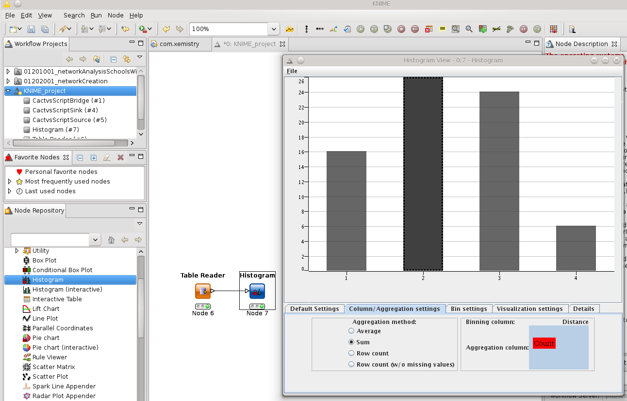
Without an explicit format specification, the output format is identified via the file name suffix. This table can be read with the standard KNIME table reader and that one directly connected to the standard barchart renderer:
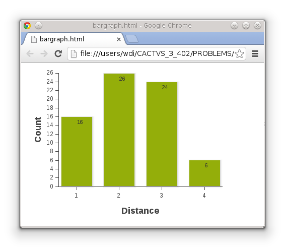
But using KNIME is not the only option. The toolkit can output various graph formats from table data for the ExtJS JavaScript toolkit. Generating a simple Web page with a bar chart is simple:
prop set T_EXTJS_VISUALIZATION datatype file
prop setparam T_EXTJS_VISUALIZATION xcolumn Distance ycolumn Count style barchart htmlpage 1 \
	extjspath http://85.214.192.197/edit filename bargraph.html
table get $th T_EXTJS_VISUALIZATION
Property T_EXTJS_VISUALIZATION has the specical capability that it can be configured to use either the property datatype blob or file. Its default blob is an in-memory data area, which is useful when constructing more complex Web pages, or direclty writing to sockets or standard output channels, since it does use the file system. In our example, we change it to file to obtain a disk file instead. Alternatively, it would of course also be possible to write the blob data to a file with a few additional lines of Tcl script code.
A few of the ExtJS visualization parameters are adjusted in the next statement. Their meaning should be obvious. with a few exeptions. For the sake of portability, the ÉxtJS installation we are referencing here is that of the Xemistry Web Sketcher. Setting the htmlpage boolean parameter instructs the computation function to output a simple but complete Web page. By default, only the JavaScript code for the actual graph is returned, which is intended to be used as a component in more complex page designs.
The final table get command then returns the specified file name, and, as a side effect, writes the file. It looks like this in a Web browser:
This tutorial requires toolkit version 3.411 or later to fully reproduce the examples. Earlier versions miss the integer matrix property datatype support and the ExtJS graph generator table property. The explained general toolkit principles are however applicable to all reasonably recent toolkit versions.